PyTorch Tensor Operations

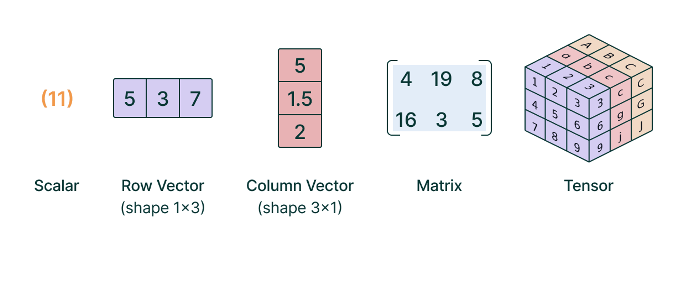
Tensors are multi-dimensional arrays that generalize scalars, vectors, and matrices to higher dimensions. In PyTorch, tensors serve as the fundamental building block for storing data and performing operations within machine learning models.
Tensor algebra is a branch of mathematics dealing with tensors and their mathematical operations. PyTorch provides numerous functionalities to manipulate and operate on tensors efficiently.

Scalar and Tensor Operations

To perform arithmetic operations between a scalar and a tensor, you simply apply the operation to each value in the tensor. For instance:

   

where is a scalar. Similarly, for scalar multiplication:

   

Element-wise Tensor Operations

To add or multiply two tensors element-wise, they must have the same shape or be compatible through a process called broadcasting. Broadcasting is an implicit mechanism by which smaller arrays are virtually expanded to match the shape of the larger array during operations, without incurring additional memory overhead.
For example, if and are two tensors of the same shape, their sum is computed as:

   

   

Only tensors with the same shape can be added directly. However, PyTorch supports adding tensors of different shapes if they can be broadcasted to a common shape.
The same principle applies to element-wise multiplication:

   

Broadcasting Example

Consider adding (or multiplying) a tensor of shape and a tensor of shape . During the addition operation, is broadcasted along the second dimension to match the shape of :

   

The resulting sum is:

   

Rearranging Tensors

Rearranging the shape of a tensor, also known as a reshape operation, does not alter the number of elements within the tensor. Instead, the total number of elements must remain constant.
For instance, a tensor with shape can be rearranged into a tensor of shape or :

   

PyTorch uses row-major tensor algebra, which implies that, when rearranging, elements are ordered from left to right starting from the first (row) dimension. The rearrange operation in PyTorch can be performed using either the reshape or view methods.

• reshape: Actually rearranges the tensor data in memory. This is a slower rearrange operation but results in faster access.
• view: Only modifies the indexing without changing the underlying memory layout. This is a fast rearrange operation, but it may result in slightly slower access during computation.

Reduction Operations

In a reduction operation, the elements of a tensor are combined together along a specific dimension to produce a new tensor with reduced dimensions. Common reduction operations include:

• sum: Computes the sum of elements along a specified dimension.
• mean: Computes the average of elements along a specified dimension.
• max and min: Find the maximum or minimum value along a specified dimension.
• std: Computes the standard deviation of elements along a specified dimension.
  For example, consider a tensor of shape :

   

We can perform a reduction along the rows (dimension 0) or along the columns (dimension 1):

   

Reduction operations are useful for summarizing data and extracting key statistics from tensors.

Matrix Multiplication

Matrix multiplication is a binary operation that takes two matrices and produces another matrix. In PyTorch, this operation can be performed using the matmul or operator.
The number of columns in the first matrix must be equal to the number of rows in the second matrix for matrix multiplication to be valid. If is of shape and is of shape , then their product will have the shape , built as follows:

   

For example:

   

Matrix multiplication is a fundamental operation in many machine learning models, particularly in fully connected and convolutional neural networks.

Tensor Initialization

There are several ways to initialize a tensor in PyTorch, each useful for different scenarios:

• From a list or NumPy array: You can create a tensor directly from a Python list or a NumPy array using the torch.tensor() function.
• Using torch.ones(shape): Initializes a tensor with all elements equal to one.
• Using torch.zeros(shape): Initializes a tensor with all elements equal to zero.
• Using random values: torch.rand(shape) generates a tensor with random values uniformly distributed between 0 and 1.
  For example:

     

  Initialization is a crucial step in neural network training as it influences the speed of convergence and the quality of the final solution.

Autograd and Backpropagation

PyTorch provides an automatic differentiation library called Autograd, which is a fundamental tool for training neural networks. It calculates the gradients of tensors with respect to a loss function, which is essential for optimizing the parameters of a model.
To enable gradient tracking, you need to set requires_grad=True when creating a tensor:

x = torch.tensor([1.0, 2.0, 3.0], requires_grad=True)

Once you have performed some operations on tensors, you can call backward() on the final tensor to compute the gradients:

y = x.sum()
y.backward()
print(x.grad)  % Outputs: tensor([1., 1., 1.])

In this example, represents a scalar value which is the sum of all elements of . The function can be thought of as a simple loss function. When we call y.backward(), PyTorch computes the gradient of with respect to each element of .

Since is defined as the sum of all elements in , we have:

   

The partial derivative of with respect to each element of is , because increasing any single element of by a small amount results in an identical increase in . Thus, x.grad will be tensor([1., 1., 1.]).
In a typical machine learning scenario, would represent a loss function that measures how far off our model’s predictions are from the true values. The backward() function calculates how we need to adjust each parameter of the model (in this case, the elements of ) to reduce this loss. The gradients stored in x.grad tell us the direction and magnitude of the change needed to minimize .

Optimization in PyTorch

In PyTorch, optimization algorithms are used to adjust the weights of the model to minimize the loss function. The torch.optim package provides several optimization algorithms, including:

• SGD: Stochastic Gradient Descent.
• Adam: Adaptive Moment Estimation, which combines the benefits of
  both SGD with momentum and RMSProp.
• Adagrad, RMSprop, etc.
  A typical optimization loop looks like this:

optimizer = torch.optim.SGD(model.parameters(), lr=0.01)
for epoch in range(num_epochs):
    optimizer.zero_grad()   # Zero the gradient buffers
    output = model(input)
    loss = loss_fn(output, target)
    loss.backward()
    optimizer.step()        # Update parameters

This loop is repeated for a number of epochs until the model converges to a suitable solution.

Data Loading with DataLoader

In PyTorch, the DataLoader class provides an easy and efficient way to load data in batches for training. This is especially important when working with large datasets, as loading the entire dataset at once may not fit into memory.
DataLoader works seamlessly with both map-style and iterable-style datasets. A typical usage example is:

from torch.utils.data import DataLoader

train_loader = DataLoader(dataset=train_dataset, batch_size=32, shuffle=True)
for batch in train_loader:
    inputs, labels = batch
    output = model(inputs)
    loss = loss_fn(output, labels)
    # Perform backward and optimization steps here

The arguments commonly passed to DataLoader include:

• dataset: The dataset from which data will be loaded.
• batch_size: Number of samples per batch to load.
• shuffle: Whether to shuffle the data at every epoch.
• num_workers: Number of subprocesses to use for data loading.
  Batching the data not only helps in better utilization of the hardware (especially GPUs), but also smoothens the optimization process by providing a better approximation of the gradient direction.

Building a Custom Dataset

In PyTorch, the Dataset class provides an abstraction for accessing and manipulating data. You can create a custom dataset by subclassing torch.utils.data.Dataset and overriding the __len__() and __getitem__() methods. Here is an example of a custom dataset:

import torch
from torch.utils.data import Dataset

class CustomDataset(Dataset):
    def __init__(self, data, labels):
        self.data = data
        self.labels = labels
    def __len__(self):
        return len(self.data)
    def __getitem__(self, idx):
        x = self.data[idx]
        y = self.labels[idx]
        return x, y

# Example usage
data = torch.randn(100, 10)  # 100 samples, 10 features each
labels = torch.randint(0, 2, (100,))  # 100 labels (binary classification)
dataset = CustomDataset(data, labels)

The key components of a custom dataset are:

• __init__(): Initializes the dataset object, often loading or generating the data.
• __len__(): Returns the number of samples in the dataset.
• __getitem__(): Given an index, returns the corresponding data sample and label.
  Custom datasets are particularly useful when working with data that is not in standard formats or needs preprocessing before training.

Using IterableDataset

In PyTorch, there are two types of dataset abstractions:

• torch.utils.data.Dataset: Follows the map-style data model, where data is accessed via indexing.
• torch.utils.data.IterableDataset: Follows the iterable-style data model, that is useful when data cannot be indexed or is generated on the fly.
  When using torch.utils.data.IterableDataset, you must implement the method __iter__() to return an iterable over the dataset. This method is typically used for streaming large datasets or generating data dynamically. For simplicity and to reduce potential errors, it is common practice to make the dataset class itself an iterator by implementing both the __iter__() and __next__() methods. This approach allows for iterating through the data points one by one.
  IterableDataset is especially useful in scenarios where the data size is too large to fit into memory or when the dataset is not predefined but generated in real-time.

Modules in PyTorch

Modules are the building blocks for creating neural networks in PyTorch. The base class for all modules is torch.nn.Module. A module can represent a single layer or a more complex model consisting of many layers.
To create a custom neural network, you define a class that inherits from nn.Module and implement at least two methods:

• __init__(): Defines the layers that will be used.
• forward(x): Defines how the data passes through the layers to produce an output.
  Here’s an example of a simple neural network model:

import torch
import torch.nn as nn
import torch.nn.functional as F

class SimpleNN(nn.Module):
    def __init__(self):
        super(SimpleNN, self).__init__()
        self.fc1 = nn.Linear(10, 50)  # Fully connected layer, input size 10, output size 50
        self.fc2 = nn.Linear(50, 1)   # Fully connected layer, input size 50, output size 1

    def forward(self, x):
        x = F.relu(self.fc1(x))  # Apply ReLU activation after the first layer
        x = self.fc2(x)          # Apply the second layer without activation
        return x

# Creating the model
model = SimpleNN()

Key Methods of the Module Class

• Initialization (__init__): Used to define the layers of the network. In the example above, fc1 and fc2 are fully connected layers.
• Forward() Defines the forward pass of the data through the various layers of the module. For instance, is passed through fc1, then the activation function (ReLU) is applied, and finally is passed through fc2.
• Accessing Parameters: All parameters of the layers (weights and biases) can be accessed via model.parameters(), which is useful for passing the object to torch.optim for optimization.

Training a Module

To train a module, you follow these main steps:

1. Define a Model: Create an instance of your custom model class.
2. Define a Loss Function: Choose an appropriate loss function, e.g., Mean Squared Error (MSE) or Cross Entropy Loss.
3. Define an Optimizer: Choose an optimization algorithm, e.g., Stochastic Gradient Descent (SGD) or Adam.
4. Training Loop: Iterate over the data, perform the forward pass, compute the loss, backpropagate the gradients, and update the weights.
   Here’s an example of a simple training loop:

import torch.optim as optim

# Create the model
model = SimpleNN()

# Define the loss function and optimizer
loss_fn = nn.MSELoss()
optimizer = optim.SGD(model.parameters(), lr=0.01)

# Training loop
for epoch in range(100):
	for batch in train_loader:
        # Forward pass
        outputs = model(batch.input)
        loss = loss_fn(outputs, batch.target)

        # Backward pass
        optimizer.zero_grad()  # Zero the gradient buffers
        loss.backward()        # Compute gradients
        optimizer.step()       # Update the parameters

    print(f'Epoch [{epoch+1}/100], Loss: {loss.item()}')

In this training loop:

• Forward Pass: The inputs are passed through the model to get the outputs.
• Loss Calculation: The difference between the model’s predictions and the true targets is computed using the loss function.
• Backward Pass: The gradients of the loss are computed with respect to each parameter.
• Optimizer Step: The parameters are updated using the optimizer and the computed gradients.
  These core elements of PyTorch’s Module class are what allow you to build, train, and extend complex neural network architectures in an efficient and flexible manner.

Simple Linear Regression in PyTorch

Linear regression models the relationship between a dependent variable and an independent variable with a linear function:

   

Where is the weight (slope) and is the bias (intercept). Here’s an example of how to implement a basic linear regression model:

import torch
import torch.nn as nn

class LinearRegressionModel(nn.Module):
    def __init__(self):
        super(LinearRegressionModel, self).__init__()
        self.linear = nn.Linear(1, 1)  # One input feature, one output feature
        
    def forward(self, x):
        return self.linear(x)

To train the model, we use a standard training loop with a loss function and an optimizer, such as Stochastic Gradient Descent (SGD).

model = LinearRegressionModel()
criterion = nn.MSELoss()  # Mean Squared Error Loss
optimizer = torch.optim.SGD(model.parameters(), lr=0.01)

# Training loop
for epoch in range(1000):  # Number of epochs
    optimizer.zero_grad()  # Zero gradients
    outputs = model(inputs)  # Forward pass
    loss = criterion(outputs, targets)  # Calculate loss
    loss.backward()  # Backward pass
    optimizer.step()  # Update weights

This implementation demonstrates how to define, train, and optimize a simple linear regression model in PyTorch.

Loss Functions in PyTorch

Training a model means computing an error (a scalar function), computing the gradient of the error w.r.t. the model parameters and following the direction that minimize the error.
PyTorch has some commonly used error functions (also called loss functions) already implemented, for example:

• Mean Absolute Error (MAE): torch.nn.L1Loss – Measures the average absolute difference between predicted and actual values. Less sensitive to outliers compared to MSE.
• Mean Squared Error (MSE): torch.nn.MSELoss – Measures the average squared difference between predicted and actual values. Suitable for tasks like predicting numerical values.
• Cross-Entropy: torch.nn.CrossEntropyLoss – Ideal for problems where each sample belongs to one class. Measures the cross-entropy between predicted and target distributions